Grids and maps

Volumetric grid

Macromolecular models are often accompanied by 3D data on an evenly spaced, rectangular grid. The data may represent electron density, a mask of the protein area, or any other scalar data.

In Gemmi such a data is stored in a class called Grid. Actually, it is a set of classes for storing different types of data: floating point numbers, integers or boolean masks. These classes also store:

• unit cell dimensions (so the grid nodes can be assigned atomic coordinates),

• and crystallographic symmetry (that determines which points on the grid are equivalent under the symmetry).

If the symmetry is not set (or is set to P1) then we effectively have a box with periodic boundary conditions.

C++

The gemmi/grid.hpp header defines:

template<typename T=float> struct Grid;

which stores dimensions and data:

int nu, nv, nw;
std::vector<T> data;

The data point can be accessed with:

T Grid<T>::get_value(int u, int v, int w) const
void Grid<T>::set_value(int u, int v, int w, T x)

The unit cell and symmetry:

UnitCell unit_cell;
const SpaceGroup* spacegroup;

can be accessed directly, except that unit_cell should be set using Grid<T>::set_unit_cell().

Unit cell parameters enable conversion between coordinates and grid points. To get an interpolated value at any position (in either fractional or orthogonal coordinates), use:

T Grid<T>::interpolate_value(const Fractional& fctr) const
T Grid<T>::interpolate_value(const Position& ctr) const

We also have a few more specialized functions. For example, a member function used primarily for masking area around atoms:

void Grid<T>::set_points_around(const Position& ctr, double radius, T value)

To make it more efficient, the function above does not consider symmetry. At the end, we should call one of the symmetrizing functions. In this case, if two symmetry-related grid point have values 0 and 1 we want to set both to 1. It can be done by calling:

void Grid<T>::symmetrize_max()

This illustrates how the Grid is meant to be used. For more information consult the source code or contact the author.

Python

Let us create a new grid:

>>> import gemmi
>>>
>>> grid = gemmi.FloatGrid(12, 12, 12)
>>> grid.set_value(1, 1, 1, 7.0)
>>> grid.get_value(1, 1, 1)
7.0
>>> # we can test wrapping of indices (a.k.a. periodic boundary conditions)
>>> grid.get_value(-11, 13, 25)
7.0

The main advantage of Grid over generic 3D arrays is that it understands crystallographic symmetry.

>>> grid.spacegroup = gemmi.find_spacegroup_by_name('P2')
>>> grid.set_value(0, 0, 0, 0.125)  # a special position
>>> grid.sum()  # for now only two points: 7.0 + 0.125
7.125
>>> grid.symmetrize_max()  # applying symmetry
>>> grid.sum()  # one point got duplicated, the other is on rotation axis
14.125
>>> for point in grid:
...   if point.value != 0.: print(point)
<gemmi.FloatGridPoint (0, 0, 0) -> 0.125>
<gemmi.FloatGridPoint (1, 1, 1) -> 7>
<gemmi.FloatGridPoint (11, 1, 11) -> 7>

The point that you get when iterating over grid has four properties:

>>> grid.get_point(0, 0, 0)
<gemmi.FloatGridPoint (0, 0, 0) -> 0.125>
>>> _.u, _.v, _.w, _.value
(0, 0, 0, 0.125)

The point can also be converted to index and to fractional and orthoghonal c oordinates, as will be demonstrated later.

The data can be also acesssed through the buffer protocol. It means that you can use it as a NumPy array (Fortran-style contiguous) without copying the data:

>>> import numpy
>>> array = numpy.array(grid, copy=False)
>>> array.dtype
dtype('float32')
>>> array.shape
(12, 12, 12)
>>> numpy.argwhere(array == 7.0)
array([[ 1,  1,  1],
       [11,  1, 11]])

(It does not make gemmi dependent on NumPy – gemmi talks with NumPy through the buffer protocol, and it can talk with any other Python library that supports this protocol.)

We may be interested only in selected part of the map. For this, we have MaskedGrid that combines two Grid objects, using one of them as a mask for the other.

When an element of the mask is 0 (false), the corresponding element of the other grid is unmasked and is to be used. The same convention is used in numpy MaskedArray.

The primary use for MaskedGrid is working with asymmetric unit (asu) only:

>>> asu = grid.asu()
>>> asu  
<gemmi.MaskedFloatGrid object at 0x...>
>>> asu.grid is grid
True
>>> asu.mask
<gemmi.Int8Grid(12, 12, 12)>
>>> sum(point.value for point in asu)
7.125
>>> for point in asu:
...   if point.value != 0: print(point)
<gemmi.FloatGridPoint (0, 0, 0) -> 0.125>
<gemmi.FloatGridPoint (1, 1, 1) -> 7>

To convert a point to index or to fractional coordinates use:

>>> point = grid.get_point(6, 6, 6)
>>> grid.point_to_index(point)
942
>>> grid.point_to_fractional(point)
<gemmi.Fractional(0.5, 0.5, 0.5)>

In addition to the symmetry, Grid may also have associated unit cell.

>>> grid.set_unit_cell(gemmi.UnitCell(45, 45, 45, 90, 82.5, 90))
>>> grid.unit_cell
<gemmi.UnitCell(45, 45, 45, 90, 82.5, 90)>

This allows us to translate location on the grid to position in Angstroms:

>>> grid.point_to_position(point)
<gemmi.Position(25.4368, 22.5, 22.3075)>

And the other way around. We can translate position in Angstroms to the location in grid, and get an interpolated value (with trilinear interpolation) at any point:

>>> grid.interpolate_value(gemmi.Position(2, 3, 4))
2.0333263874053955

This function can also take fractional position:

>>> grid.interpolate_value(gemmi.Fractional(1/24, 1/24, 1/24))
0.890625

If you need to interpolate values at so many points on a regular 3D grid that calling interpolate_value() for each point would be too slow, use interpolate_values() (with s at the end) instead. It takes a 3D numpy array and a Transform that relates indices of the array to positions in the grid, and fills the array with the interpolated values:

>>> # first we create a numpy array of the same type as the grid
>>> arr = numpy.zeros([32, 32, 32], dtype=numpy.float32)
>>> # then we setup a transformation (array indices) -> (position [A]).
>>> tr = gemmi.Transform()
>>> tr.mat.fromlist([[0.1, 0, 0], [0, 0.1, 0], [0, 0, 0.1]])
>>> tr.vec.fromlist([1, 2, 3])
>>> grid.interpolate_values(arr, tr)
>>> arr[10, 10, 10]  # -> corresponds to Position(2, 3, 4)
2.0333264

If you would like to set grid points near a specified position use the set_points_around() function:

>>> grid.set_points_around(gemmi.Position(25, 25, 25), radius=3, value=10)
>>> numpy.argwhere(array == 10)
array([[6, 6, 7],
       [6, 7, 7]])
>>> # now the data does not obey symmetry, we should call symmetrize*()

To set all point values, do:

>>> grid.fill(1.23)

MRC/CCP4 maps

We support one file format for storing the grid data on disk: MRC/CCP4 map. The content of the map file is stored in a class that contains both the Grid class and all the meta-data from the CCP4 file header.

The CCP4 format has a few different modes that correspond to different data types. Gemmi supports:

• mode 0 – which correspond to the C++ type int8_t,

• mode 1 – corresponds to int16_t,

• mode 2 – float,

• and mode 6 – uint16_t.

CCP4 programs use mode 2 (float) for the electron density, and mode 0 (int8_t) for masks. Mask is 0/1 data that marks part of the volume (e.g. the solvent region). Other modes are not used in crystallography, but may be used for CryoEM data.

The CCP4 format is quite flexible. The data is stored as sections, rows and columns that correspond to a permutation of the X, Y and Z axes as defined in the file header. The file can contain only a part of the asymmetric unit, or more than an asymmetric unit (i.e. redundant data). There are two typical approaches to generate a crystallographic map:

• old-school way: a map covering a molecule with some margin around it is produced using CCP4 utilities such as fft and mapmask,

• or a map is made for the asymmetric unit (asu), and the program that reads the map is supposed to expand the symmetry. This approach is used by the CCP4 clipper library and by programs that use this library, such as cfft and Coot.

The latter approach generates map for exactly one asu, if possible. It is not possible if the shape of the asu in fractional coordinates is not rectangular, and in such case we must have some redundancy. On average, the maps generated for asu are significantly smaller, as compared in the UglyMol wiki.

Nowadays, the CCP4 format is rarely used in crystallography. Almost all programs read the reflection data and calculate maps on the fly.

C++

Reading

To read and write CCP4 maps you need:

#include <gemmi/ccp4.hpp>

We normally use float type when reading a map file:

gemmi::Ccp4<float> map;
map.read_ccp4_map("my_map.ccp4");

and int8_t when reading a mask (mask typically has only values 0 and 1, but in principle it can have values from -127 to 128):

gemmi::Ccp4<int8_t> mask;
mask.read_ccp4_map("my_mask.ccp4");

If the grid data type does not match the file data type, the library will attempt to convert the data when reading.

Header

The CCP4 map header is organised as 56 words followed by space for ten 80-character text labels. The member functions that access the data from the map header use the word number (as in the format description) as a location in the header:

int32_t header_i32(int w) const;
float header_float(int w) const;
// ccp4 map header has mostly 80-byte strings
std::string header_str(int w, size_t len=80) const;

void set_header_i32(int w, int32_t value);
void set_header_float(int w, float value);
void set_header_str(int w, const std::string& str);

For example:

int mode = map.header_i32(4);
float x = map.header_float(11);

setup()

read_ccp4_map() stores the data as it is written in the file. In many situation, it is convenient to have the data expanded to the whole unit cell, with axes in a specific order (X, Y, Z is the most conventional one). For this we have a function:

map.setup(GridSetup::Full, NAN);  // unknown values are set to NAN

This call is required to make grid functions work correctly with the unit cell parameters.

Writing

To write a map to a file:

// the file header needs to be prepared/updated with an explicit call
int mode = 2; // ccp4 file mode: 2 for floating-point data, 0 for masks
bool update_stats = true; // update min/max/mean/rms values in the header
map.update_ccp4_header(mode, update_stats);

map.write_ccp4_map(filename);

Python

The Python API is similar.

>>> m = gemmi.read_ccp4_map('../tests/5i55_tiny.ccp4')
>>> m
<gemmi.Ccp4Map with grid (8, 6, 10) in SG #4>
>>> m.grid  # tiny grid as it is a toy example
<gemmi.FloatGrid(8, 6, 10)>
>>> m.grid.spacegroup
<gemmi.SpaceGroup("P 1 21 1")>
>>> m.grid.unit_cell
<gemmi.UnitCell(29.45, 10.5, 29.7, 90, 111.975, 90)>
>>> m.setup()
>>> m.grid
<gemmi.FloatGrid(60, 24, 60)>
>>> m.write_ccp4_map('out.ccp4')

For the low-level access to header one can use the same getters and setters as in the C++ version.

>>> m.header_float(20), m.header_float(21)  # dmin, dmax
(-0.5310382843017578, 2.3988280296325684)
>>> m.header_i32(28)
0
>>> m.set_header_i32(28, 20140)
>>> m.header_str(57, 80).strip()
'Created by MAPMAN V. 080625/7.8.5 at Wed Jan 3 12:57:38 2018 for A. Nonymous'

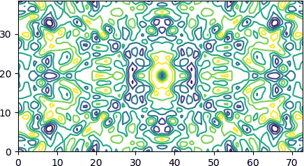
Let us end with a short code that draws a contour plot similar to mapslicer plots (see Fig. 3 in this CCP4 paper if you wonder what is mapslicer). To keep the example short we assume that the lattice vectors are orthogonal.

import numpy
from matplotlib import pyplot
import gemmi

# toxd_aupatt.map is generated by $CCP4/examples/unix/runnable/patterson
ccp4 = gemmi.read_ccp4_map('/tmp/wojdyr/toxd_aupatt.map')
ccp4.setup()
arr = numpy.array(ccp4.grid, copy=False)
x = numpy.linspace(0, ccp4.grid.unit_cell.a, num=arr.shape[0], endpoint=False)
y = numpy.linspace(0, ccp4.grid.unit_cell.b, num=arr.shape[1], endpoint=False)
X, Y = numpy.meshgrid(x, y, indexing='ij')
pyplot.contour(X, Y, arr[:,:,40])
pyplot.gca().set_aspect('equal', adjustable='box')
pyplot.show()